Checkpoint 2
Last Updated: Mar 30, 2026
Contents
- Contents
- Design Lab
- Task 2.1 Odometry-based Mapping
- Task 2.2 Localization-only
- Task 2.3 Simultaneous Localization and Mapping (SLAM)
- Checkpoint Submission
Design Lab
We’ve released the Design Lab Guide!
You need to design and build a forklift mechanism. The design file is due with your Checkpoint 2 submission, but it doesn’t need to be final, a prototype version is perfectly fine. The goal is to help you stay on track.
Designing, prototyping, and testing should continue alongside the main checkpoints until the final competition.
Task 2.1 Odometry-based Mapping
In this task, you will implement occupancy grid mapping based on odometry. For task 2.1, we will treat odometry as the ground truth for the robot’s position. You will map the environment by assuming the LiDAR sensor’s origin matches the robot’s odometry coordinates.
We publish the occupancy grid on the map frame from localization_node. Since we are assuming the odometry pose is the “real” pose, we hard-code the map -> odom transform in the launch file as a static zero transform (all zeros), the map frame and the odom frame will be perfectly overlapped in this task, effectively making the map frame our global world frame.
Spoiler alert, odometry is rarely the “real” pose in practice due to drift, but we will address how to handle those errors later.
TODO
- Check the ROB550 GitLab
mbot_ros_labsupstream to see if there is any new commits to pull. - Navigate to
mbot_ros_labs/mbot_slam/src. For Task 2.1, start withmapping_node.cpp, we define the mapping node here, then complete the logic incommon/mapping.cppandcommon/moving_laser_scan.cpp. Search TODO in all three files.
Explanation of TODOs
- Deskewing LiDAR scan in
common/moving_laser_scan.cpp- A laser scan isn’t instantaneous. The sensor rotates over a finite time interval, if the robot is moving while scanning, there will be spatial distortion. For example:
- The initial beam is captured at robot_start_pose (e.g., x=1.0, y=0).
- The last beam is captured at robor_end_pose (e.g., x=1.1, y=0).
- We have to project each beam to its true origin, and can not assume all beams in a single scan are fired from the same position.
- To account for this, the
MovingLaserScanclass performs deskewing. When initialized, it calculates an interpolated beam pose for each individual beam between the scan_start_pose and scan_end_pose. ThescanCallbackfunction already handles these 2 poses. And you need to implement the interpolation logic within the MovingLaserScan::deskewScan function to populate the corrected ray origins and headings.
- A laser scan isn’t instantaneous. The sensor rotates over a finite time interval, if the robot is moving while scanning, there will be spatial distortion. For example:
- Bresenham’s algorithm in
common/mapping.cpp- After interpolating all rays, use Bresenham’s algorithm to determine which cells in the occupancy grid each ray passes through.
- Update map cells in
common/mapping.cppandmapping_node.cpp- For each beam, update the corresponding cells using log-odds to reflect occupancy probabilities.
When finished, compile your code:
cd ~/mbot_ros_labs
colcon build --packages-select mbot_slam
source install/setup.bash
- Important: You must source the workspace in every relevant terminal after each build. If you don’t, ROS will keep using the old code, and your changes will not take effect.
ROS bag test
What is a ros bag? - A ros bag is like a recorder for ROS data, saves topic messages such as odometry, LiDAR scans, and TF.
- We provide a rosbag recorded on the instructor’s MBot that includes all data needed for mapping. You can replay it on any machine even without a robot, to test your mapping node. This lets you isolate other variables and focus purely on your mapping logic.
- If mapping works with the rosbag, your mapping logic is correct. But real-world results may vary since odometry depends on your robot’s firmware, for example, the instructor’s MBot implemented gyrodometry.
All the data required for this task comes from the ROS bag, you DO NOT need to manually publish anything.
- Unplug USB-C cable between Pi and Pico, the ros bag contains
/cmd_velyour mbot will drive away. - Run the following in the VSCode Terminal to start the mapping node:
cd ~/mbot_ros_labs source install/setup.bash ros2 launch mbot_slam mapping.launch.py - Visualization, either thru NoMachine
 # on NoMachine terminal
 cd ~/mbot_ros_labs/src/mbot_slam/rviz
 ros2 run rviz2 rviz2 -d mapping.rviz
OR Foxglove
# Launch foxglove bridge using vscode terminal ros2 launch foxglove_bridge foxglove_bridge_launch.xml - Play the rosbag in the VSCode Terminal
 cd ~/mbot_ros_labs/src/mbot_rosbags
 ros2 bag play slam_test
Tip: If your map looks similar to the map in demo video, that’s a good result, small errors are expected.
Real world test
- Check all the wires are connected, put the robot in the maze you want to map, reset the odometry,
- Run the following in VSCode Terminal #1 to launch the lidar driver, robot tf tree, robot model:
ros2 launch mbot_bringup mbot_bringup.launch.py - Run the following in the VSCode Terminal #2 to start the mapping node:
cd ~/mbot_ros_labs source install/setup.bash ros2 launch mbot_slam mapping.launch.py - Using teleop control to move the robot in the maze, run in VSCode Terminal #3:
ros2 run teleop_twist_keyboard teleop_twist_keyboard - Visualization, either thru NoMachine
 # on NoMachine terminal
 cd ~/mbot_ros_labs/src/mbot_slam/rviz
 ros2 run rviz2 rviz2 -d mapping.rviz
or Foxglove
# Launch foxglove bridge using vscode terminal ros2 launch foxglove_bridge foxglove_bridge_launch.xml - After mapping the whole area, do not stop the mapping node yet. Save the map if you want to, in VSCode Terminal:
cd ~/mbot_ros_labs/src/mbot_slam/maps ros2 run nav2_map_server map_saver_cli -f your_map_name- Replace
map_namewith the name you want for your map. - After saving, you can stop the mapping node.
- Replace
To view the map after saving:
- Option 1: Use a local viewer. Install a VSCode extension like PGM Viewer to open your map file.
- Option 2: Publish the map in ROS2
cd ~/mbot_ros_labs # we need to re-compile so the launch file can find the newly saved map colcon build --packages-select mbot_slam source install/setup.bash ros2 launch mbot_slam view_map.launch.py map_name:=your_map_name- This will publish the map to the
/maptopic. - You can now view it in RViz (via NoMachine) or Foxglove Studio.
- This will publish the map to the
Include a screenshot of your map. Analyze the map quality and explain why it is not ideal.
Task 2.2 Localization-only
Monte Carlo Localization (MCL) is a particle-filter-based localization algorithm. To implement MCL, you need three key components:
- Action model: predicts the robot’s next pose.
- Sensor model: calculates the likelihood of a pose given a sensor measurement.
- Particle filter functions: draw samples, normalize particle weights, and compute the weighted mean pose.
TODO
- All work for this task is in the package
mbot_slam.- Start with
localization_node.cpp, find out where we call particle filter. - Then move to
particle_filter.cpp, understand how we use action model and sensor model there, search for TODO. - Check
action_model.cppandsensor_model.cpp, search for TODO.
- Start with
- When finished, compile your code:
cd ~/mbot_ros_labs colcon build --packages-select mbot_slam source install/setup.bash- Important: You must source the workspace in every relevant terminal after each build. If you don’t, ROS will keep using the old code, and your changes will not take effect.
ROS bag test
For Task 2.2, we only use the provided rosbag, no real-world test is needed. This task focuses on localization, which requires a reliable map. Using the rosbag saves time from remapping the maze and eliminates variables that could affect localization performance, such as a poor map. All the data required for this task comes from the ROS bag, you DO NOT need to manually publish anything.
The localization node publishes both the estimated path and the reference path, your estimated path shouldn’t be too off from the reference. If your output looks similar to the demo video, it’s good enough.
- This ROS bag includes the
/cmd_veltopic, unplug the Type-C cable from the Pi to the Pico to prevent the robot from driving away. - Visualization, either thru NoMachine
 # On NoMachine
 cd ~/mbot_ros_labs/src/mbot_slam/rviz
 ros2 run rviz2 rviz2 -d localization.rviz
or Foxglove
# Launch foxglove bridge using vscode terminal ros2 launch foxglove_bridge foxglove_bridge_launch.xml - Run the localization node in the VSCode Terminal:
cd ~/mbot_ros_labs source install/setup.bash # When use rosbag, publish_tf should be false ros2 run mbot_slam localization_node --ros-args -p publish_tf:=false - Play the ROS bag in the VSCode Terminal:
 cd ~/mbot_ros_labs/src/mbot_rosbags/maze1
 ros2 bag play maze1.mcap
1) Report in a table the time it takes to update the particle filter for 100, 500 and 1000 particles. Estimate the maximum number of particles your filter can support running at 10Hz.
2) Include a screenshot comparing your estimated pose path with the reference pose path.
Task 2.3 Simultaneous Localization and Mapping (SLAM)
You have now implemented mapping using known poses and localization using a known map. You can now implement the following simple SLAM algorithm:
- Use the first laser scan received to construct an initial map.
- For subsequent laser scans:
- Localize using the map from the previous iteration.
- Update the map using the pose estimate from your localization.
TODO
- All work for this task is in the
mbot_slampackage. Start withslam_node.cppand search for TODOs in updateGrid(). The logic should matchmapping.cpp, so you can copy and paste it.- Good news: you already implemented everything needed in Tasks 2.1 and 2.2, so you can compile and start testing.
- However, you might see the result is not great yet. This is because we still need to tune the parameters; details are below.
- When finished, compile your code:
cd ~/mbot_ros_labs colcon build --packages-select mbot_slam source install/setup.bash- Important: You must source the workspace in every relevant terminal after each build. If you don’t, ROS will keep using the old code, and your changes will not take effect.
If your mapping and localization are working well, but your full SLAM system is struggling, the problem is often in parameter tuning. Here are some hints to guide your tuning:
- Action model
action_model.hpp- Observe your particle cloud: What is its shape? Is it a tight circle, or an elongated oval following the robot’s path? If
k2_ork1_is too high, your particle cloud might be a “long oval”. - We know the robot’s odometry isn’t perfect, but it’s also not completely wrong. Is a large noise value like 1.0 necessary, or would a much smaller value like 0.001 be more appropriate? Think about how much you trust the odometry.
- Observe your particle cloud: What is its shape? Is it a tight circle, or an elongated oval following the robot’s path? If
- Mapping
mapping.hpp- Do you see cells “flickering” between free and occupied? This can happen if a few bad scans can erase a well-defined wall. Tune the log-odds limits: Consider tunning
kMaxLogOddsandkMinLogOdds. to make it harder for a cell’s state to be “flipped” after it’s been confidently marked as occupied or free.
- Do you see cells “flickering” between free and occupied? This can happen if a few bad scans can erase a well-defined wall. Tune the log-odds limits: Consider tunning
ROS bag test
- Visualization, either thru NoMachine
 cd ~/mbot_ros_labs/src/mbot_slam/rviz
 ros2 run rviz2 rviz2 -d slam.rviz
or Foxglove
# Launch foxglove bridge using vscode terminal ros2 launch foxglove_bridge foxglove_bridge_launch.xml - Start the SLAM Node in VSCode Terminal:
cd ~/mbot_ros_labs source install/setup.bash ros2 run mbot_slam slam_node - Play the ros bag. This ROS bag includes the
/cmd_veltopic, unplug the Type-C cable from the Pi to the Pico to prevent the robot from driving away.cd ~/mbot_ros_labs/src/mbot_rosbags ros2 bag play slam_test
Real world test
- Check all the wires are connected, put the robot in the maze you want to map, reset the odometry,
- Visualization, either thru NoMachine
 cd ~/mbot_ros_labs/src/mbot_slam/rviz
 ros2 run rviz2 rviz2 -d slam.rviz
or Foxglove
# Launch foxglove bridge using vscode terminal ros2 launch foxglove_bridge foxglove_bridge_launch.xml - Run the following in VSCode Terminal:
ros2 launch mbot_bringup mbot_bringup.launch.py - Start the SLAM Node in VSCode Terminal:
cd ~/mbot_ros_labs source install/setup.bash ros2 run mbot_slam slam_node - Drive the robot manually using the teleop in VSCode Terminal:
ros2 run teleop_twist_keyboard teleop_twist_keyboard - After mapping the whole area, do not stop the mapping node yet. Save the map if you want to, in VSCode Terminal:
cd ~/mbot_ros_labs/src/mbot_slam/maps ros2 run nav2_map_server map_saver_cli -f your_map_name- Replace
map_namewith the name you want for your map. - After saving, you can stop the mapping node.
- Replace
Here are examples of “OK,” “Good,” and “Excellent” maps generated from the slam_test bag. These are related to how competition scoring will be evaluated.
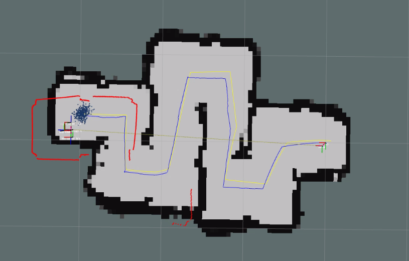
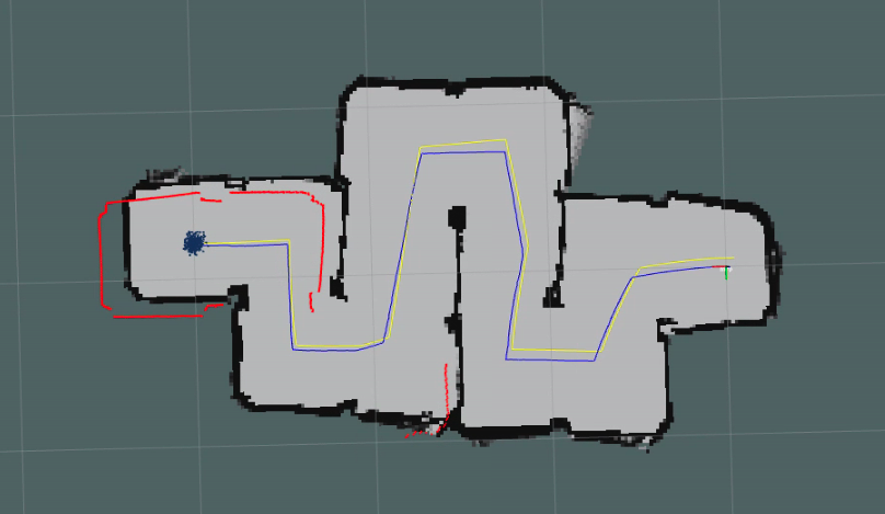
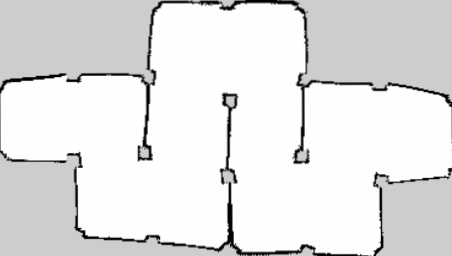
1) Create a block diagram showing how the SLAM system components interact.
2) Include a screenshot of your map, and explain why your SLAM-generated map is better than the one from Task 2.1.
Checkpoint Submission
Demonstrate your SLAM system by mapping the maze used in Checkpoint 1. You may either manually drive the robot using teleop or use the motion controller from Checkpoint 1.
- Submit a screenshot of the generated map.
- Submit the map file itself.
- Submit a short description of your SLAM system, including how it works and any key observations.
- Submit your forklift design prototype, it can be in any form, such as a simple sketch, a CAD file, or other representation.